6.10 ridge plot

# sphinx_gallery_thumbnail_number = 2

import numpy as np
import pandas as pd
from easy_mpl import ridge
import matplotlib.pyplot as plt
from easy_mpl.utils import version_info

version_info()  # print version information of all the packages being used

{'easy_mpl': '0.21.4', 'matplotlib': '3.8.4', 'numpy': '1.26.4', 'pandas': '1.5.3', 'scipy': '1.13.1'}

data_ = np.random.random(size=100)
_ = ridge(data_)

data_ = np.random.random((100, 3))
_ = ridge(data_)

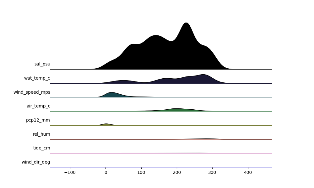
specifying colormap

_ = ridge(data_, color="Blues")

The data can also be in the form of pandas DataFrame

_ = ridge(pd.DataFrame(data_))

if we don’t want to fill the ridge, we can specify the color as white

_ = ridge(np.random.random(100), color=["white"])

we can draw all the ridges on same axes as below

df = pd.DataFrame(np.random.random((100, 3)), dtype='object')
_ = ridge(df, share_axes=True, fill_kws={"alpha": 0.5})

we can also provide an existing axes to plot on

_, ax = plt.subplots()
_ = ridge(df, ax=ax, fill_kws={"alpha": 0.5})

The data can also be in the form of list of arrays

x1 = np.random.random(100)
x2 = np.random.random(100)
_ = ridge([x1, x2], color=np.random.random((3, 2)))

The length of arrays need not to be constant/same. We can use arrays of different lengths

x1 = np.random.random(100)
x2 = np.random.random(90)
_ = ridge([x1, x2], color=np.random.random((3, 2)))

f = "https://raw.githubusercontent.com/AtrCheema/AI4Water/master/ai4water/datasets/arg_busan.csv"
df = pd.read_csv(f, index_col='index')
print(df.shape)
df.head()

(1446, 25)

	tide_cm	wat_temp_c	sal_psu	air_temp_c	pcp_mm	...	aac_coppml	Total_otus	otu_5575	otu_273	otu_94
index
6/19/2018 0:00	36.407149	19.321232	33.956058	19.780000	0.0	...	NaN	NaN	NaN	NaN	NaN
6/19/2018 0:30	35.562515	19.320124	33.950508	19.093333	0.0	...	NaN	NaN	NaN	NaN	NaN
6/19/2018 1:00	34.808016	19.319666	33.942532	18.733333	0.0	...	NaN	NaN	NaN	NaN	NaN
6/19/2018 1:30	30.645216	19.320406	33.931263	18.760000	0.0	...	NaN	NaN	NaN	NaN	NaN
6/19/2018 2:00	26.608980	19.326729	33.917961	18.633333	0.0	...	NaN	NaN	NaN	NaN	NaN

5 rows × 25 columns

cols = ['air_temp_c',
        'wat_temp_c',
        'sal_psu',
        'tide_cm',
        'rel_hum',
        'pcp12_mm',
        'wind_dir_deg',
        'wind_speed_mps'
        ]

_ = ridge(df[cols])

f = 'https://media.githubusercontent.com/media/HakaiInstitute/essd2021-hydromet-datapackage/main/2013-2019_Discharge1015_5min.csv'
df = pd.read_csv(f)
df.index = pd.to_datetime(df.pop('Datetime'))
print(df.shape)
df.head()

(543568, 12)

	Watershed	Qlevel	Qflag	Qrate	Qrate_min	...	Qvol_min	Qvol_max	Qmm	Qmm_min	Qmm_max
Datetime
2014-07-31 13:50:00+00:00	WTS1015	2	AV	0.0442	0.0025	...	0.75	29.85	0.004	0.0002	0.009
2014-07-31 13:55:00+00:00	WTS1015	2	AV	0.0442	0.0025	...	0.75	29.85	0.004	0.0002	0.009
2014-07-31 14:00:00+00:00	WTS1015	2	AV	0.0442	0.0025	...	0.75	29.85	0.004	0.0002	0.009
2014-07-31 14:05:00+00:00	WTS1015	2	AV	0.0442	0.0025	...	0.75	29.85	0.004	0.0002	0.009
2014-07-31 14:10:00+00:00	WTS1015	2	AV	0.0442	0.0025	...	0.75	29.85	0.004	0.0002	0.009

5 rows × 12 columns

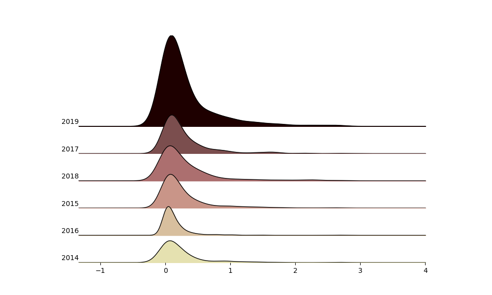
groupby_year = df.groupby(lambda x: x.year)

_ = ridge(
    [grp['Qrate'].resample('D').interpolate(method='linear') for _, grp in groupby_year],
    labels=[name for name, _ in groupby_year],
    )