6.13 spider plot
Note
Click here to download the full example code or to run this example in your browser via Binder
6.13 spider plot#
# sphinx_gallery_thumbnail_number = -2

import numpy as np
import pandas as pd
import matplotlib.pyplot as plt
from easy_mpl import spider_plot
from easy_mpl.utils import version_info, create_subplots

version_info()
{'easy_mpl': '0.21.4', 'matplotlib': '3.8.4', 'numpy': '1.26.4', 'pandas': '1.5.3', 'scipy': '1.13.1'}

specifying labels

# specifying tick size

# specifying colors on our own
# specifying outline color

# we can also specify cmap in place of color
Using dataframe
df = pd.DataFrame.from_dict(
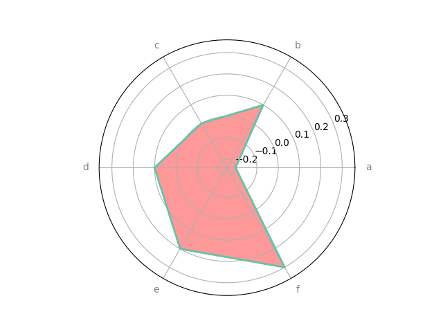
{'summer': {'a': -0.2, 'b': 0.1, 'c': 0.0, 'd': 0.1, 'e': 0.2, 'f': 0.3},
'winter': {'a': -0.3, 'b': 0.1, 'c': 0.0, 'd': 0.2, 'e': 0.15,'f': 0.25}})
_ = spider_plot(df, xtick_kws={'size': 20})
# #%%
df = pd.DataFrame.from_dict(
{'summer': {'a': -0.2, 'b': 0.1, 'c': 0.0, 'd': 0.1, 'e': 0.2, 'f': 0.3},
'winter': {'a': -0.3, 'b': 0.1, 'c': 0.0, 'd': 0.2, 'e': 0.15, 'f': 0.25},
'automn': {'a': -0.1, 'b': 0.3, 'c': 0.15, 'd': 0.24, 'e': 0.18, 'f': 0.2}})
_ = spider_plot(df, xtick_kws={'size': 20})
# #%%
# use polygon frame
_ = spider_plot(data=values, frame="polygon")


_ = spider_plot(df, xtick_kws={'size': 20}, frame="polygon",
           color=['b', 'r', 'g', 'm'],
            fill_color=['b', 'r', 'g', 'm'])

postprocessing of axes
df = pd.DataFrame.from_dict(
    {
        'Hg (Adsorption)': {'1': 97.4, '2': 92.38, '3': 81.2, '4': 73.2, '5': 66.81},
        'Cd (Adsorption)': {'1': 96.2, '2': 91.1, '3': 80.02, '4': 71.55, '5': 64.8},
        'Pb (Adsorption)': {'1': 92.7, '2': 86.3, '3': 78.4, '4': 71.2, '5': 64.4},
        'Hg (Desorption)': {'1': 97.6, '2': 96.5, '3': 94.1, '4': 91.99, '5': 90.0},
        'Cd (Desorption)': {'1': 97.0, '2': 96.2, '3': 94.7, '4': 93.7, '5': 92.5},
        'Pb (Desorption)': {'1': 97.0, '2': 95.8, '3': 93.7, '4': 91.8, '5': 89.9}
     })

_ = spider_plot(df, frame="polygon",
            fill_kws = {"alpha": 0.0},
            xtick_kws={'size': 14, "weight": "bold", "color": "black"},
            show=False,
            leg_kws = {'bbox_to_anchor': (0.90, 1.1)}
            )

plt.gca().set_rmax(100.0)
plt.gca().set_rmin(60.0)
plt.gca().set_rgrids((60.0, 70.0, 80.0, 90.0, 100.0),
                     ("60%", "70%", "80%", "90%", "100%"),
                     fontsize=14, weight="bold", color="black"),
plt.tight_layout()
plt.show()

matplotlib example
data = [
    ['Sulfate', 'Nitrate', 'EC', 'OC1', 'OC2', 'OC3', 'OP', 'CO', 'O3'],
    ('Basecase', [
        [0.88, 0.01, 0.03, 0.03, 0.00, 0.06, 0.01, 0.00, 0.00],
        [0.07, 0.95, 0.04, 0.05, 0.00, 0.02, 0.01, 0.00, 0.00],
        [0.01, 0.02, 0.85, 0.19, 0.05, 0.10, 0.00, 0.00, 0.00],
        [0.02, 0.01, 0.07, 0.01, 0.21, 0.12, 0.98, 0.00, 0.00],
        [0.01, 0.01, 0.02, 0.71, 0.74, 0.70, 0.00, 0.00, 0.00]]),
    ('With CO', [
        [0.88, 0.02, 0.02, 0.02, 0.00, 0.05, 0.00, 0.05, 0.00],
        [0.08, 0.94, 0.04, 0.02, 0.00, 0.01, 0.12, 0.04, 0.00],
        [0.01, 0.01, 0.79, 0.10, 0.00, 0.05, 0.00, 0.31, 0.00],
        [0.00, 0.02, 0.03, 0.38, 0.31, 0.31, 0.00, 0.59, 0.00],
        [0.02, 0.02, 0.11, 0.47, 0.69, 0.58, 0.88, 0.00, 0.00]]),
    ('With O3', [
        [0.89, 0.01, 0.07, 0.00, 0.00, 0.05, 0.00, 0.00, 0.03],
        [0.07, 0.95, 0.05, 0.04, 0.00, 0.02, 0.12, 0.00, 0.00],
        [0.01, 0.02, 0.86, 0.27, 0.16, 0.19, 0.00, 0.00, 0.00],
        [0.01, 0.03, 0.00, 0.32, 0.29, 0.27, 0.00, 0.00, 0.95],
        [0.02, 0.00, 0.03, 0.37, 0.56, 0.47, 0.87, 0.00, 0.00]]),
    ('CO & O3', [
        [0.87, 0.01, 0.08, 0.00, 0.00, 0.04, 0.00, 0.00, 0.01],
        [0.09, 0.95, 0.02, 0.03, 0.00, 0.01, 0.13, 0.06, 0.00],
        [0.01, 0.02, 0.71, 0.24, 0.13, 0.16, 0.00, 0.50, 0.00],
        [0.01, 0.03, 0.00, 0.28, 0.24, 0.23, 0.00, 0.44, 0.88],
        [0.02, 0.00, 0.18, 0.45, 0.64, 0.55, 0.86, 0.00, 0.16]])
]

fig, axes = create_subplots(4, subplot_kw= dict(projection='polar'),
                            figsize=(8,8))

spoke_labels = data.pop(0)
labels = ('Factor 1', 'Factor 2', 'Factor 3', 'Factor 4', 'Factor 5')

for ax, (title, col) in zip(axes.flat, data):

    d = np.array(col).transpose()
    ax.set_title(title, fontdict={'fontsize': 14, 'fontweight':'bold'})
    _ = spider_plot(d, show=False, ax=ax,
                    tick_labels=spoke_labels, xtick_kws=dict(size=12)
                    )

    ax.tick_params(axis='x', which='major', pad=12)
    ax.set_facecolor('floralwhite')

fig.legend(labels, loc='center', labelspacing=0.1, fontsize='large')
plt.tight_layout()
plt.show()

Total running time of the script: ( 0 minutes 5.063 seconds)